Beautiful plots while simulating loss in two-part Procrustes problem

Today, I was working on a two part Procrustes problem and wanted to find out why my minimization algorithm sometimes does not converge properly or renders unexpected results. The loss function to be minimized is

$$L(\mathbf{Q},c)=\parallel c{\mathbf{A}}_{\mathbf{1}}\mathbf{Q}-{\mathbf{B}}_{\mathbf{1}}{\parallel }^2+\parallel {\mathbf{A}}_{\mathbf{2}}\mathbf{Q}-{\mathbf{B}}_{\mathbf{2}}{\parallel }^2\to min$$

with $\parallel \cdot \parallel$ denoting the Frobenius norm, $c$ is an unknown scalar and $\mathbf{Q}$ an unknown rotation matrix, i.e. ${\mathbf{Q}}^T\mathbf{Q}=\mathbf{I}$. ${\mathbf{A}}_{\mathbf{1}},{\mathbf{A}}_{\mathbf{2}},{\mathbf{B}}_{\mathbf{1}}$, and ${\mathbf{B}}_{\mathbf{1}}$ are four real valued matrices. The minimum for $c$ is easily found by partial derivation and setting to zero.

$$c=\frac{tr{\mathbf{Q}}^T{{\mathbf{A}}_{\mathbf{1}}}^T{\mathbf{B}}_{\mathbf{1}}}{\parallel {\mathbf{A}}_{\mathbf{1}}{\parallel }^2}$$

By plugging $c$ into the loss function $L(\mathbf{Q},c)$ we get a new loss function $L(\mathbf{Q})$ that only depends on $\mathbf{Q}$. This is the starting situation.

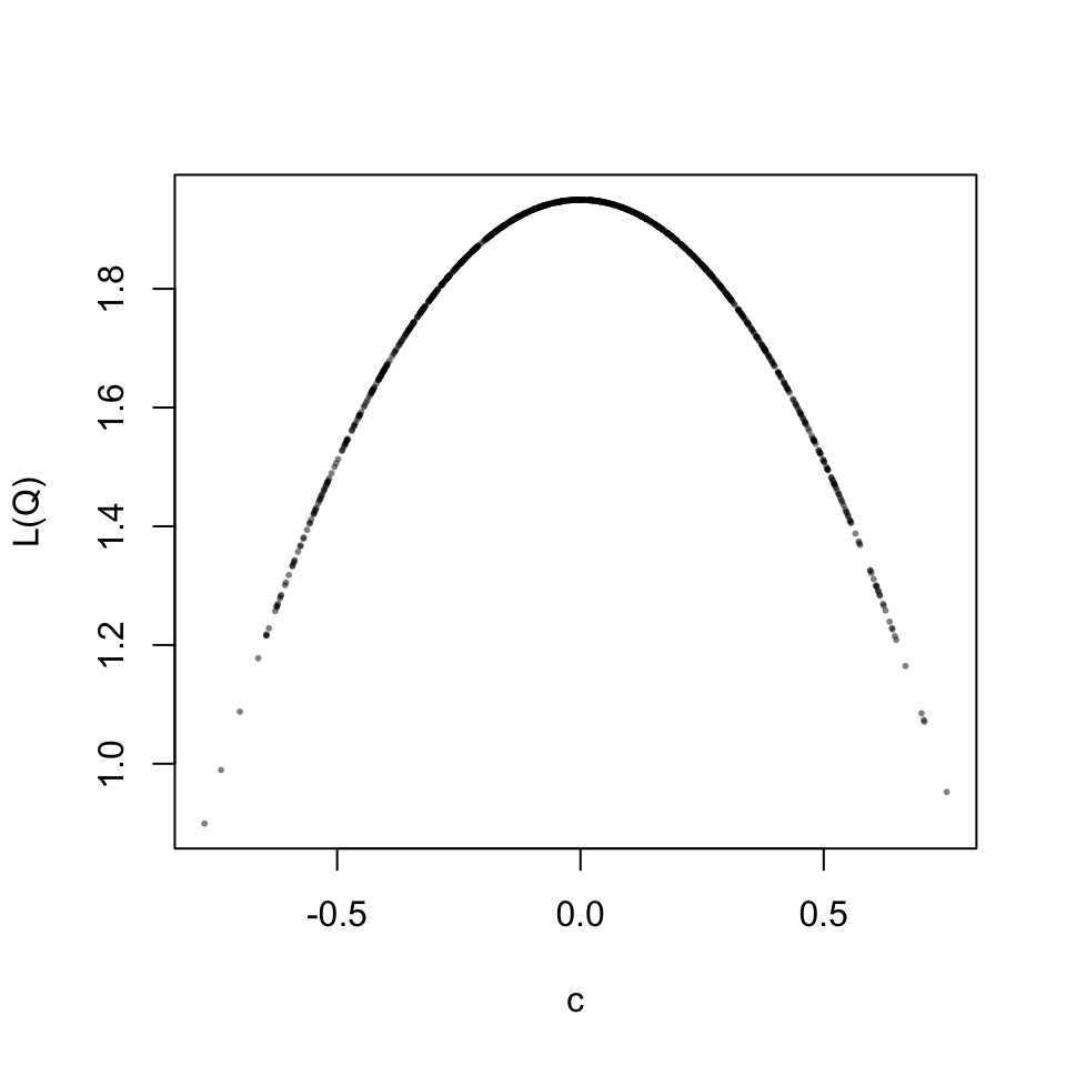
When trying to find out why the algorithm to minimize $L(\mathbf{Q})$ did not work as expected, I got stuck. So I decided to conduct a small simulation and generate random rotation matrices to study the relation between the parameter $c$ and the value of the loss function $L(\mathbf{Q})$. Before looking at the results, let’s visualize the results for the first part of the above Procrustes problem, with $c$ having the same solution as before.

$$L(\mathbf{Q},c)=\parallel c{\mathbf{A}}_{\mathbf{1}}\mathbf{Q}-{\mathbf{B}}_{\mathbf{1}}{\parallel }^2\to min$$

This is a well behaved relation, for each scaling parameter the loss value is identical. Now let’s look at the full two-part loss function. The result turns out to be beautiful.

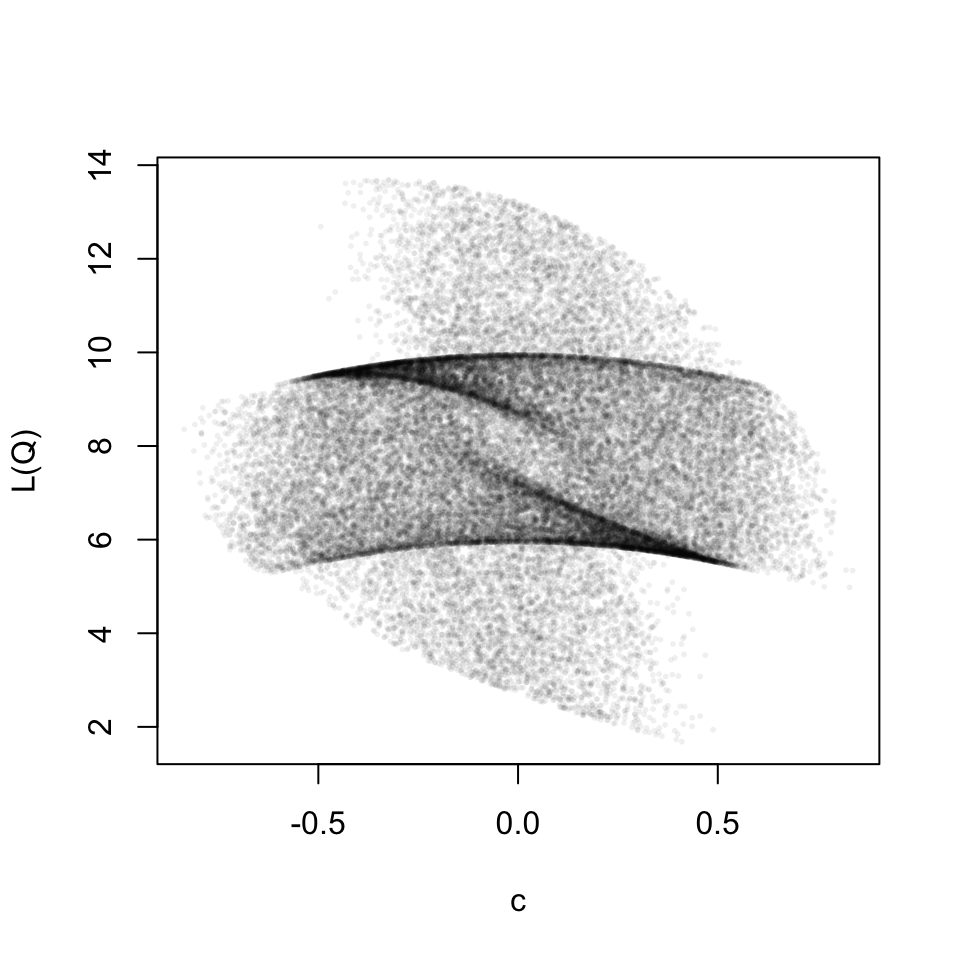
For the graphic above I used the following matrices.

$$A1=\left(\begin{array}{ccc}0.0& 0.4& -0.5\\ -0.4& -0.8& -0.5\\ -0.1& -0.5& 0.2\end{array}\right),B1=\left(\begin{array}{ccc}-0.1& -0.8& -0.1\\ 0.3& 0.2& -0.9\\ 0.1& -0.3& -0.5\end{array}\right)$$ $$A2=\left(\begin{array}{ccc}1& 0& 0\\ 0& 0& 1\\ 0& 1& 0\end{array}\right),B2=\left(\begin{array}{ccc}0& 1& 0\\ 1& 0& 0\\ 0& 0& 1\end{array}\right)$$

And the following R-code.

tr <- function(X) sum(diag(X))

# random matrix type 1
rmat_1 <- function(n=3, p=3, min=-1, max=1){
  matrix(runif(n*p, min, max), ncol=p)
}

# random matrix type 2, sparse
rmat_2 <- function(p=3) {
  diag(p)[, sample(1:p, p)]
}

# generate random rotation matrix Q. Based on Q find 
# optimal scaling factor c and calculate loss function value
#
one_sample <- function(n=2, p=2)
{
  Q <- mixAK::rRotationMatrix(n=1, dim=p) %*%         # random rotation matrix
    diag(sample(c(-1,1), p, rep=T))                   # additionally 
  s <- tr( t(Q) %*% t(A1) %*% B1 ) / norm(A1, "F")^2  # scaling factor c
  rss <- norm(s*A1 %*% Q - B1, "F")^2 + 
         norm(A2 %*% Q - B2, "F")^2 
  c(s=s, rss=rss)
}

# find c and rss or many random rotation matrices
#
set.seed(10)  # nice case for 3 x 3
n <- 3
p <- 3
A1 <- round(rmat_1(n, p), 1)
B1 <- round(rmat_1(n, p), 1)
A2 <- rmat_2(p)
B2 <- rmat_2(p)

x <- rdply(40000, one_sample(3,3)) 
plot(x$s, x$rss, pch=16, cex=.4, xlab="c", ylab="L(Q)", col="#00000010")

Below you find some more graphics with different matrices as inputs.

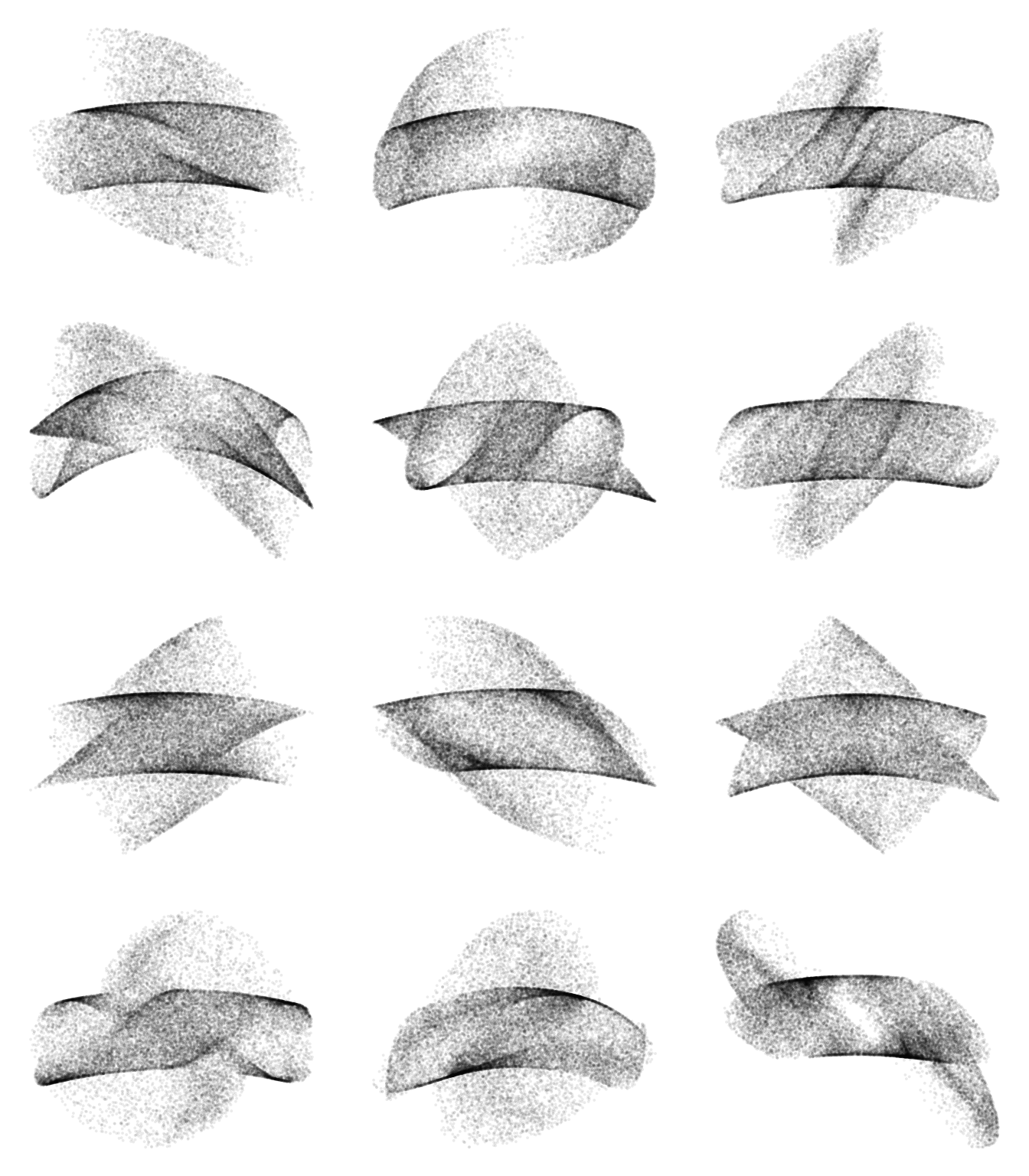
Here, we do not have a one-to-one relation between the scaling parameter and the loss function any more. I do not quite know what to make of this yet. But for now I am happy that it has aesthetic value.