Regression - Custom parameter hypotheses

Introduction

When performing a regression, the default output in most statistical programs tests every parameter against the null hypothesis that the population parameters equals zero, i.e. there is no effect. Yet, in many cases this is not what we want. We may need to specify custom hypotheses like the following: Does the parameter $b_1$ equal $1$ ? Are parameters $b_1$ and $b_2$ equal? In this document we will briefly outline how to test such hypotheses for regression parameters in R. Let’s start by creating a dataset.

set.seed(1)
S <- c(1, .3, .8,                        # create covariance matrix for sample data
      .3,  1, .5, 
      .8, .5, 1)
Sigma <- matrix(S, ncol=3, by=T)
n <- 10
x <- mvrnorm(n = n, mu=c(0,0,0), Sigma)  # multivariate normally distributed data
d <- as.data.frame(x)

# dependent variable Y as linear combination plus error
d <- transform(d, Y = scale(V1) + scale(V2) + scale(V3) + rnorm(n, sd=.5))

Next, we will estimate a regression model and output the coefficientes. The function summary returns several results for a regression model. We are only interested in the coefficients. The summary object s is made up of several smaller objects (type names(s)). One contains the a dataframe of estimated coefficients.

m <- lm(Y ~ V1 + V2, data=d)
s <- summary(m)
b <- s$coefficients
b   # b is a dataframe with coefficients

              Estimate Std. Error   t value     Pr(>|t|)
(Intercept) -0.4826666  0.2133013 -2.262840 5.808762e-02
V1           2.3944398  0.2928401  8.176612 7.926576e-05
V2           0.7642977  0.1952398  3.914661 5.788626e-03

The standard test statistic, as given in the output, tests the default hypothesis of a zero effect, i.e. ${\beta }_{H_0}=0$. The corresponding test statistic for the t-Test is

$t=\frac{\hat{\beta }-{\beta }_{H_0}}{\text{s.e.}(\hat{\beta })}$.

To retrieve the estimate, standard error (s.e.), t- and p-value for a coefficient, you can access the dataframe b, e.g. for V1.

b["V1",]

    Estimate   Std. Error      t value     Pr(>|t|) 
2.394440e+00 2.928401e-01 8.176612e+00 7.926576e-05 

Before we will test custom hypotheses, let’s reproduce the t- and p-value step by step, to get a better understanding of what happens.

b_h0 <- 0                       # null hypothesis
b_hat <- b[1,1]                 # estimate for V1
b_se <- b[1,2]                  # s.e. for V1
ts <- (b_hat - b_h0) / b_se     # test statistic, i.e. t-value
deg <- m$df.residual            # degrees of freedom of residual, i.e. 10-3
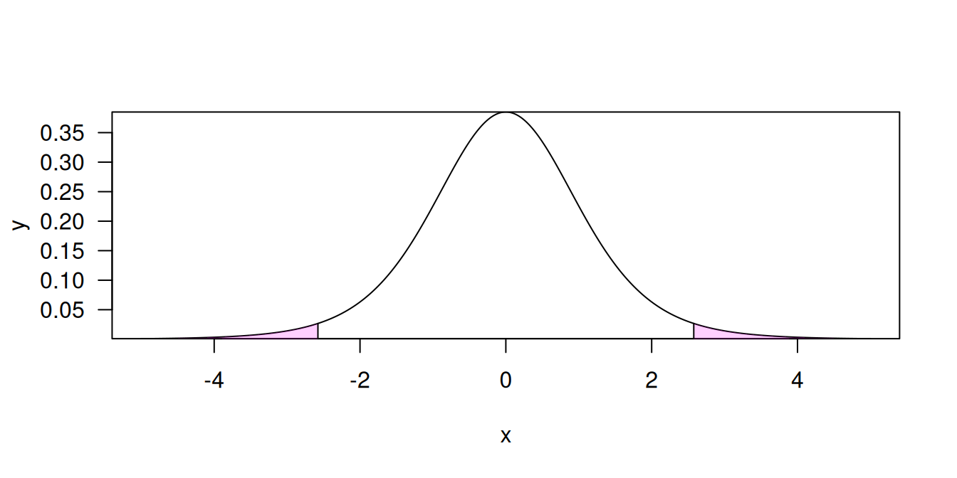
2*pt(abs(ts), deg, lower=FALSE) # note that it is a two sided test, hence 2 x ...

[1] 0.05808762

As the test is two-sided, the t-value (test value) cuts off a region of the t-distribution at both ends. The size of the region equals the p-value.

Testing if a parameter has a specific value

Now our goal is to test another hypothesis, not the default that the population parameter is equal to zero. There are several ways how to do that in R. We will explore three ways.

1. t-Test

The first approach is straighforward. To test against another value than zero, we merely need to change the null hypothesis of the t-Test. E.g. to test if the coefficient $\beta$ deviates from $1$, we use the same test statistic as above but with ${\beta }_{H_0}=1$.

b_h0 <- 1                         # null hypothesis
ts <- (b_hat - b_h0) / b_se       # test statistic, i.e. t-value
2*pt(abs(ts), deg, lower=FALSE)   # note that it is a two sided test

[1] 0.0002209872

For convencience, we can wrap the code into a function that allows to select a coefficient and specify a custom null hypothesis value.

# m:        lm model object
# b.index:  index of model parameter to test
# b_h0:     hypothesis to test parameter against
#
test_h0 <- function(m, b.index, b_h0)
{
  b <- summary(m)$coef            # get coefficients
  ts <- (b[b.index, 1] - b_h0) / 
         b[b.index, 2]            # test statistic, i.e. t-value
  deg <- m$df.residual            # degrees of freedom of residual
  2*pt(abs(ts), deg, lower=FALSE) # note that it is a two sided test
}

Let’s test our function.

test_h0(m, 1, 1)

[1] 0.0002209872

2. Comparing a model and a linearily restricted model

Another way to achieve the same is to compare our model to a linearily restricted model. This test allows to test multiple hypotheses on multiple parameters. We can e.g. test hypotheses like ${\beta }_1={\beta }_2$ or ${\beta }_1+{\beta }_2=1$. The function linearHypothesis from the car package performs a test for hypotheses of this kind. The argument hypothesis.matrix takes a matrix, where every row specifies a linear combination of parameters. The argument rhs takes the right-hand-side, i.e. the results of this combination. In our case we want to specify the hypothesis that ${\beta }_0=1$.

h <- linearHypothesis(m, hypothesis.matrix = c(1, 0, 0), rhs=1)
h

Linear hypothesis test

Hypothesis:
(Intercept) = 1

Model 1: restricted model
Model 2: Y ~ V1 + V2

  Res.Df     RSS Df Sum of Sq      F   Pr(>F)    
1      8 21.4282                                 
2      7  2.7116  1    18.717 48.317 0.000221 ***
---
Signif. codes:  0 '***' 0.001 '**' 0.01 '*' 0.05 '.' 0.1 ' ' 1

Note that the p-value is exactly the same as in the t-Test before.

3. Reparametrization

A third way to test this hypothesis is to slightly rewrite the regression model. This process is called reparametrization. Let $\theta ={\beta }_1-1$ and $\theta +1={\beta }_1$. Then the hypothesis that $\theta$ equals zero is equivalent to ${\beta }_1-1=0$, i.e. ${\beta }_1=1$. This means we can use the standard regression output (which tests the default hypothesis that a parameter is zero) if we rewrite the model to include $\theta$. To rewrite the model, replace ${\beta }_1$ by $\theta +1$.

$$y={\beta }_0+{\beta }_{1}V1+{\beta }_{2}V2$$ $$y={\beta }_0+(\theta +1)V1+{\beta }_{2}V2$$ $$y-V1={\beta }_0+\theta V1+{\beta }_{2}V2$$

We can now use this new parametrization to get what we want.

m2 <- lm(I(Y - 1) ~ V1 + V2, data=d)
summary(m2)$coef

              Estimate Std. Error   t value     Pr(>|t|)
(Intercept) -1.4826666  0.2133013 -6.951044 2.209872e-04
V1           2.3944398  0.2928401  8.176612 7.926576e-05
V2           0.7642977  0.1952398  3.914661 5.788626e-03

Again note that the p-value for $\theta$ equals the above results. Also, note that the estimate for $\theta$ is the same as subtracting $1$ from the estimate for ${\beta }_1$ from the original model, i.e. $-0.4826666-1=-1.4826666$. The only advantage is that by this approach we also get the standard error for $\theta$ and can thus perform a test. For this simple hypothesis the s.e. is the same anyway. For more complicated hypotheses this will however not be the case.

More complicated hypotheses

We may be interested in testing more complicated hypothesis. E.g. if the effect of two parameters is identical i.e. if ${\beta }_1={\beta }_2$. Using linearHypothesis this is straighforward. Just reformulate the hypothesis to get a scalar value on the right hand side, i.e. ${\beta }_1-{\beta }_2=0$. Now we can plug the hypothesis into the function.

h <- linearHypothesis(m, hypothesis.matrix = c(0, 1, -1), rhs=0)
h

Linear hypothesis test

Hypothesis:
V1 - V2 = 0

Model 1: restricted model
Model 2: Y ~ V1 + V2

  Res.Df    RSS Df Sum of Sq      F   Pr(>F)   
1      8 8.7382                                
2      7 2.7116  1    6.0266 15.558 0.005572 **
---
Signif. codes:  0 '***' 0.001 '**' 0.01 '*' 0.05 '.' 0.1 ' ' 1

Again reparametrization can be used as well. Let $\theta$ be the difference between the two coefficients, i.e. ${\beta }_1-{\beta }_2=\theta$. Now we can test if $\theta$ is zero using the default regression output. To rewrite our model we use ${\beta }_1=\theta +{\beta }_2$ and insert it into the regression formula.

$$y={\beta }_0+{\beta }_{1}V1+{\beta }_{2}V2$$ $$y={\beta }_0+(\theta +{\beta }_2)V1+{\beta }_{2}V2$$ $$y={\beta }_0+\theta V1+{\beta }_2(V1+V2)$$

m3 <- lm(Y ~ V1 + I(V1 + V2), data=d)
b3 <- summary(m3)$coef
b3

              Estimate Std. Error   t value    Pr(>|t|)
(Intercept) -0.4826666  0.2133013 -2.262840 0.058087619
V1           1.6301421  0.4132873  3.944332 0.005572322
I(V1 + V2)   0.7642977  0.1952398  3.914661 0.005788626

The estimate for $\theta$, i.e. the difference between ${\beta }_1$ and ${\beta }_2$ is 1.6301. The corresponding p-value for the hypothesis that difference between them is zero is 0.006. Again note, that the value is the same as above.

Deriving standard errors for combinations of parameters

Another approach to conduct a statistical test is it to derive the standard error for the weighted parameter combination $\theta$ we want to test from the variance-covariance matrix of the regression parameters.

Let $\theta$ be a weighted combination of parameters.

$$\theta =\sum _{j=1}^k{\lambda }_j{\beta }_j$$

Then the standard error of $\theta$ is

$$s_{\theta }^2=\sum _{j=1}^k{\lambda }_j^2{s}_{{\beta }_j}^2+2\sum _{j\ne i}^k{\lambda }_j{\lambda }_i{s}_{{\beta }_{j}i}$$

The s.e. for any combinations of parameters can also be derived from the estimates of the parameter’s s.e. Let’s get the estimated regression parameters variance / covariance matrix.

cm <- vcov(m)
cm

             (Intercept)          V1           V2
(Intercept)  0.045497437 -0.02368300  0.009120892
V1          -0.023682995  0.08575533 -0.023466238
V2           0.009120892 -0.02346624  0.038118573

The combination we are interested in is $\theta =1\cdot {\beta }_1+(-1)\cdot {\beta }_2$, i.e. ${\lambda }_1=1$ and ${\lambda }_2=-1$. The estimated standard error for $\theta$ thus is

s2.theta <- sum(1^2*cm[2,2] + (-1)^2*cm[3,3]) + 2*sum(1*(-1)*cm[2,3])
s.theta = s2.theta^.5
s.theta

[1] 0.4132873

Note that the value matches the result from the approach above. We can now perform a t-test using this result for the s.e. The results are already shown in the regression output from the reparametrization above. But for the sake of completeness we will do it here once more by hand.

b_h0 <- 0                           # null hypothesis
ts <- (b3[2, 1] - b_h0) / s.theta   # test statistic, i.e. t-value
2*pt(abs(ts), deg, lower=FALSE)     # note that it is a two sided test

[1] 0.005572322

Note, that the value is equal to the p-value shown in the regression output from the reparametrization above.